Computations for Potential density, buoyancy and geostrophic shear
contribution of Hemant Khatri.
[1]:
import xarray as xr
from xgcm import Grid
import numpy as np
import matplotlib.pyplot as plt
import matplotlib.cm as cm
import warnings

warnings.filterwarnings("ignore")
%matplotlib inline
First load the usual MOM6 dataset with xarray:
[2]:
dataurl = 'http://35.188.34.63:8080/thredds/dodsC/OM4p5/'

ds = xr.open_dataset(f'{dataurl}/ocean_monthly_z.200301-200712.nc4',
                     chunks={'time':1, 'z_l': 1}, engine='pydap')
[3]:
ds
[3]:
<xarray.Dataset>
Dimensions:       (nv: 2, time: 60, xh: 720, xq: 720, yh: 576, yq: 576, z_i: 36, z_l: 35)
Coordinates:
  * nv            (nv) float64 1.0 2.0
  * xh            (xh) float64 -299.8 -299.2 -298.8 -298.2 ... 58.75 59.25 59.75
  * xq            (xq) float64 -299.5 -299.0 -298.5 -298.0 ... 59.0 59.5 60.0
  * yh            (yh) float64 -77.91 -77.72 -77.54 -77.36 ... 89.47 89.68 89.89
  * yq            (yq) float64 -77.82 -77.63 -77.45 -77.26 ... 89.58 89.79 90.0
  * z_i           (z_i) float64 0.0 5.0 15.0 25.0 ... 5.75e+03 6.25e+03 6.75e+03
  * z_l           (z_l) float64 2.5 10.0 20.0 32.5 ... 5.5e+03 6e+03 6.5e+03
  * time          (time) object 2003-01-16 12:00:00 ... 2007-12-16 12:00:00
Data variables:
    Coriolis      (yq, xq) float32 dask.array<chunksize=(576, 720), meta=np.ndarray>
    areacello     (yh, xh) float32 dask.array<chunksize=(576, 720), meta=np.ndarray>
    areacello_bu  (yq, xq) float32 dask.array<chunksize=(576, 720), meta=np.ndarray>
    areacello_cu  (yh, xq) float32 dask.array<chunksize=(576, 720), meta=np.ndarray>
    areacello_cv  (yq, xh) float32 dask.array<chunksize=(576, 720), meta=np.ndarray>
    deptho        (yh, xh) float32 dask.array<chunksize=(576, 720), meta=np.ndarray>
    dxCu          (yh, xq) float32 dask.array<chunksize=(576, 720), meta=np.ndarray>
    dxCv          (yq, xh) float32 dask.array<chunksize=(576, 720), meta=np.ndarray>
    dxt           (yh, xh) float32 dask.array<chunksize=(576, 720), meta=np.ndarray>
    dyCu          (yh, xq) float32 dask.array<chunksize=(576, 720), meta=np.ndarray>
    dyCv          (yq, xh) float32 dask.array<chunksize=(576, 720), meta=np.ndarray>
    dyt           (yh, xh) float32 dask.array<chunksize=(576, 720), meta=np.ndarray>
    geolat        (yh, xh) float32 dask.array<chunksize=(576, 720), meta=np.ndarray>
    geolat_c      (yq, xq) float32 dask.array<chunksize=(576, 720), meta=np.ndarray>
    geolat_u      (yh, xq) float32 dask.array<chunksize=(576, 720), meta=np.ndarray>
    geolat_v      (yq, xh) float32 dask.array<chunksize=(576, 720), meta=np.ndarray>
    geolon        (yh, xh) float32 dask.array<chunksize=(576, 720), meta=np.ndarray>
    geolon_c      (yq, xq) float32 dask.array<chunksize=(576, 720), meta=np.ndarray>
    geolon_u      (yh, xq) float32 dask.array<chunksize=(576, 720), meta=np.ndarray>
    geolon_v      (yq, xh) float32 dask.array<chunksize=(576, 720), meta=np.ndarray>
    hfgeou        (yh, xh) float32 dask.array<chunksize=(576, 720), meta=np.ndarray>
    sftof         (yh, xh) float32 dask.array<chunksize=(576, 720), meta=np.ndarray>
    thkcello      (z_l, yh, xh) float32 dask.array<chunksize=(1, 576, 720), meta=np.ndarray>
    wet           (yh, xh) float32 dask.array<chunksize=(576, 720), meta=np.ndarray>
    wet_c         (yq, xq) float32 dask.array<chunksize=(576, 720), meta=np.ndarray>
    wet_u         (yh, xq) float32 dask.array<chunksize=(576, 720), meta=np.ndarray>
    wet_v         (yq, xh) float32 dask.array<chunksize=(576, 720), meta=np.ndarray>
    average_DT    (time) timedelta64[ns] dask.array<chunksize=(1,), meta=np.ndarray>
    average_T1    (time) datetime64[ns] dask.array<chunksize=(1,), meta=np.ndarray>
    average_T2    (time) datetime64[ns] dask.array<chunksize=(1,), meta=np.ndarray>
    so            (time, z_l, yh, xh) float32 dask.array<chunksize=(1, 1, 576, 720), meta=np.ndarray>
    time_bnds     (time, nv) timedelta64[ns] dask.array<chunksize=(1, 2), meta=np.ndarray>
    thetao        (time, z_l, yh, xh) float32 dask.array<chunksize=(1, 1, 576, 720), meta=np.ndarray>
    umo           (time, z_l, yh, xq) float32 dask.array<chunksize=(1, 1, 576, 720), meta=np.ndarray>
    uo            (time, z_l, yh, xq) float32 dask.array<chunksize=(1, 1, 576, 720), meta=np.ndarray>
    vmo           (time, z_l, yq, xh) float32 dask.array<chunksize=(1, 1, 576, 720), meta=np.ndarray>
    vo            (time, z_l, yq, xh) float32 dask.array<chunksize=(1, 1, 576, 720), meta=np.ndarray>
    volcello      (time, z_l, yh, xh) float32 dask.array<chunksize=(1, 1, 576, 720), meta=np.ndarray>
    zos           (time, yh, xh) float32 dask.array<chunksize=(1, 576, 720), meta=np.ndarray>
Attributes:
    filename:                        ocean_monthly.200301-200712.zos.nc
    title:                           OM4p5_IAF_BLING_CFC_abio_csf_mle200
    associated_files:                areacello: 20030101.ocean_static.nc
    grid_type:                       regular
    grid_tile:                       N/A
    external_variables:              areacello
    DODS_EXTRA.Unlimited_Dimension:  time
Next we create the xgcm Grid object:
[4]:
grid = Grid(ds, coords={'X': {'center': 'xh', 'right': 'xq'},
                        'Y': {'center': 'yh', 'right': 'yq'},
                        'Z': {'center': 'z_l', 'outer': 'z_i'} }, periodic=['X']);
Potential density
There are several python packages for computations using the Equation Of State (e.g. gsw, seawater, xgcm/fastjmd95). Here we need the Wright 97 EOS to stay consistent with MOM6 model. In this formulation, the potential density can be expressed by:
[5]:
def pdens(S,theta):

    # --- Define constants (Table 1 Column 4, Wright 1997, J. Ocean Tech.)---
    a0 = 7.057924e-4
    a1 = 3.480336e-7
    a2 = -1.112733e-7

    b0 = 5.790749e8
    b1 = 3.516535e6
    b2 = -4.002714e4
    b3 = 2.084372e2
    b4 = 5.944068e5
    b5 = -9.643486e3

    c0 = 1.704853e5
    c1 = 7.904722e2
    c2 = -7.984422
    c3 = 5.140652e-2
    c4 = -2.302158e2
    c5 = -3.079464

    # To compute potential density keep pressure p = 100 kpa
    # S in standard salinity units psu, theta in DegC, p in pascals

    p = 100000.
    alpha0 = a0 + a1*theta + a2*S
    p0 = b0 + b1*theta + b2*theta**2 + b3*theta**3 + b4*S + b5*theta*S
    lambd = c0 + c1*theta + c2*theta**2 + c3*theta**3 + c4*S + c5*theta*S

    pot_dens = (p + p0)/(lambd + alpha0*(p + p0))

    return pot_dens
A naive approach to computing the potential density would be to pass our dataarrays directly to the function, i.e.
pot_density = pdens(ds.so, ds.thetao)If we use the function directly, the risk is that we will probably swith from lazy evaluation to eager. Instead we can wrap the function with apply_ufunc and stay in a lazy evaluation mode:
[6]:
pt = xr.apply_ufunc(pdens, ds.so, ds.thetao,
                    dask='parallelized',
                    output_dtypes=[ds.so.dtype])

print(pt)
<xarray.DataArray (time: 60, z_l: 35, yh: 576, xh: 720)>
dask.array<pdens, shape=(60, 35, 576, 720), dtype=float32, chunksize=(1, 1, 576, 720), chunktype=numpy.ndarray>
Coordinates:
  * xh       (xh) float64 -299.8 -299.2 -298.8 -298.2 ... 58.75 59.25 59.75
  * yh       (yh) float64 -77.91 -77.72 -77.54 -77.36 ... 89.47 89.68 89.89
  * z_l      (z_l) float64 2.5 10.0 20.0 32.5 ... 5e+03 5.5e+03 6e+03 6.5e+03
  * time     (time) object 2003-01-16 12:00:00 ... 2007-12-16 12:00:00
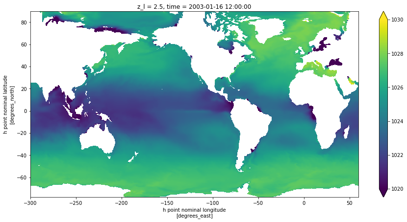
You can verify that the evaluation was instantaneous (no computation made) and we can now compute (can also use pt.compute()) and plot for one level and one time slice with:
[7]:
fig = plt.figure(figsize=(15,7))
pt.isel(z_l=0, time = 0).plot(vmin=1020, vmax=1030)
[7]:
<matplotlib.collections.QuadMesh at 0x11b6d79b0>
Buoyancy
In order to compute buoyancy, we first define reference density = 1035 kg/m\(^3\). Then we compute density anomaly as:
[8]:
rho_ref = 1035.
anom_density = pt - rho_ref
and buoyancy:
\(b = -g \frac{\rho'}{\rho_o}\)
[9]:
g = 9.81
buoyancy = -g * anom_density / rho_ref
[10]:
buoyancy
[10]:
<xarray.DataArray (time: 60, z_l: 35, yh: 576, xh: 720)>
dask.array<truediv, shape=(60, 35, 576, 720), dtype=float32, chunksize=(1, 1, 576, 720), chunktype=numpy.ndarray>
Coordinates:
  * xh       (xh) float64 -299.8 -299.2 -298.8 -298.2 ... 58.75 59.25 59.75
  * yh       (yh) float64 -77.91 -77.72 -77.54 -77.36 ... 89.47 89.68 89.89
  * z_l      (z_l) float64 2.5 10.0 20.0 32.5 ... 5e+03 5.5e+03 6e+03 6.5e+03
  * time     (time) object 2003-01-16 12:00:00 ... 2007-12-16 12:00:00
Geostrophic shear
First interpolate the Coriolis parameter onto U, V points:
[11]:
f_U = grid.interp(ds.Coriolis, 'Y', boundary='fill')
f_V = grid.interp(ds.Coriolis, 'X', boundary='fill')
Then compute density gradients in the (x,y) direction. Those are then located also on (U, V) points:
[12]:
ddens_dx = grid.diff(anom_density, 'X', boundary='fill') / ds.dxCu
ddens_dy = grid.diff(anom_density, 'Y', boundary='fill') / ds.dyCv
Finally the geostrophic shear can be expressed as:
[13]:
dz_ug =   ddens_dy * g / (f_V * rho_ref)
dz_vg = - ddens_dx * g / (f_U * rho_ref)
We can now look at the results. NB: this will trigger eager computation and may take some time to process even with a dask cluster.
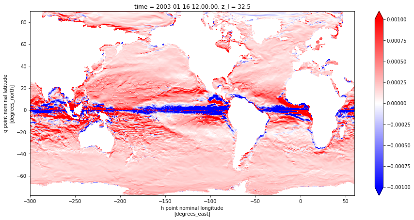
[14]:
# Geostrophic Shear plot
tmp = dz_ug.isel({'z_l': slice(3,4), 'time' : slice(0,1)})

fig = plt.figure(figsize=(15,7))
tmp.plot(cmap = 'bwr', vmin = -.001, vmax = 0.001)
[14]:
<matplotlib.collections.QuadMesh at 0x11e7da2e8>