Getting started with MOM6

• MOM6 variables are staggered according to the Arakawa C-grid

• It uses a north-east index convention

• center points are labelled (xh, yh) and corner points are labelled (xq, yq)

• important: variables xh/yh, xq/yq that are named “nominal” longitude/latitude are not the true geographical coordinates and are not suitable for plotting (more later)

See indexing for details.

import xarray as xr
from xgcm import Grid
import warnings
import matplotlib.pylab as plt
import cartopy.crs as ccrs
import cmocean

%matplotlib inline
warnings.filterwarnings("ignore")

For this tutorial, we are going to use sample data for the \(\frac{1}{2}^{\circ}\) global model OM4p05 hosted on a GFDL thredds server:

dataurl = 'http://35.188.34.63:8080/thredds/dodsC/OM4p5/'

ds = xr.open_dataset(f'{dataurl}/ocean_monthly_z.200301-200712.nc4',
                     chunks={'time':1, 'z_l': 1}, drop_variables=['average_DT',
                                                                  'average_T1',
                                                                  'average_T2'],
                     engine='pydap')

ds

<xarray.Dataset>
Dimensions:       (nv: 2, time: 60, xh: 720, xq: 720, yh: 576, yq: 576, z_i: 36, z_l: 35)
Coordinates:
  * nv            (nv) float64 1.0 2.0
  * xh            (xh) float64 -299.8 -299.2 -298.8 -298.2 ... 58.75 59.25 59.75
  * xq            (xq) float64 -299.5 -299.0 -298.5 -298.0 ... 59.0 59.5 60.0
  * yh            (yh) float64 -77.91 -77.72 -77.54 -77.36 ... 89.47 89.68 89.89
  * yq            (yq) float64 -77.82 -77.63 -77.45 -77.26 ... 89.58 89.79 90.0
  * z_i           (z_i) float64 0.0 5.0 15.0 25.0 ... 5.75e+03 6.25e+03 6.75e+03
  * z_l           (z_l) float64 2.5 10.0 20.0 32.5 ... 5.5e+03 6e+03 6.5e+03
  * time          (time) object 2003-01-16 12:00:00 ... 2007-12-16 12:00:00
Data variables:
    Coriolis      (yq, xq) float32 dask.array<chunksize=(576, 720), meta=np.ndarray>
    areacello     (yh, xh) float32 dask.array<chunksize=(576, 720), meta=np.ndarray>
    areacello_bu  (yq, xq) float32 dask.array<chunksize=(576, 720), meta=np.ndarray>
    areacello_cu  (yh, xq) float32 dask.array<chunksize=(576, 720), meta=np.ndarray>
    areacello_cv  (yq, xh) float32 dask.array<chunksize=(576, 720), meta=np.ndarray>
    deptho        (yh, xh) float32 dask.array<chunksize=(576, 720), meta=np.ndarray>
    dxCu          (yh, xq) float32 dask.array<chunksize=(576, 720), meta=np.ndarray>
    dxCv          (yq, xh) float32 dask.array<chunksize=(576, 720), meta=np.ndarray>
    dxt           (yh, xh) float32 dask.array<chunksize=(576, 720), meta=np.ndarray>
    dyCu          (yh, xq) float32 dask.array<chunksize=(576, 720), meta=np.ndarray>
    dyCv          (yq, xh) float32 dask.array<chunksize=(576, 720), meta=np.ndarray>
    dyt           (yh, xh) float32 dask.array<chunksize=(576, 720), meta=np.ndarray>
    geolat        (yh, xh) float32 dask.array<chunksize=(576, 720), meta=np.ndarray>
    geolat_c      (yq, xq) float32 dask.array<chunksize=(576, 720), meta=np.ndarray>
    geolat_u      (yh, xq) float32 dask.array<chunksize=(576, 720), meta=np.ndarray>
    geolat_v      (yq, xh) float32 dask.array<chunksize=(576, 720), meta=np.ndarray>
    geolon        (yh, xh) float32 dask.array<chunksize=(576, 720), meta=np.ndarray>
    geolon_c      (yq, xq) float32 dask.array<chunksize=(576, 720), meta=np.ndarray>
    geolon_u      (yh, xq) float32 dask.array<chunksize=(576, 720), meta=np.ndarray>
    geolon_v      (yq, xh) float32 dask.array<chunksize=(576, 720), meta=np.ndarray>
    hfgeou        (yh, xh) float32 dask.array<chunksize=(576, 720), meta=np.ndarray>
    sftof         (yh, xh) float32 dask.array<chunksize=(576, 720), meta=np.ndarray>
    thkcello      (z_l, yh, xh) float32 dask.array<chunksize=(1, 576, 720), meta=np.ndarray>
    wet           (yh, xh) float32 dask.array<chunksize=(576, 720), meta=np.ndarray>
    wet_c         (yq, xq) float32 dask.array<chunksize=(576, 720), meta=np.ndarray>
    wet_u         (yh, xq) float32 dask.array<chunksize=(576, 720), meta=np.ndarray>
    wet_v         (yq, xh) float32 dask.array<chunksize=(576, 720), meta=np.ndarray>
    so            (time, z_l, yh, xh) float32 dask.array<chunksize=(1, 1, 576, 720), meta=np.ndarray>
    time_bnds     (time, nv) timedelta64[ns] dask.array<chunksize=(1, 2), meta=np.ndarray>
    thetao        (time, z_l, yh, xh) float32 dask.array<chunksize=(1, 1, 576, 720), meta=np.ndarray>
    umo           (time, z_l, yh, xq) float32 dask.array<chunksize=(1, 1, 576, 720), meta=np.ndarray>
    uo            (time, z_l, yh, xq) float32 dask.array<chunksize=(1, 1, 576, 720), meta=np.ndarray>
    vmo           (time, z_l, yq, xh) float32 dask.array<chunksize=(1, 1, 576, 720), meta=np.ndarray>
    vo            (time, z_l, yq, xh) float32 dask.array<chunksize=(1, 1, 576, 720), meta=np.ndarray>
    volcello      (time, z_l, yh, xh) float32 dask.array<chunksize=(1, 1, 576, 720), meta=np.ndarray>
    zos           (time, yh, xh) float32 dask.array<chunksize=(1, 576, 720), meta=np.ndarray>
Attributes:
    filename:                        ocean_monthly.200301-200712.zos.nc
    title:                           OM4p5_IAF_BLING_CFC_abio_csf_mle200
    associated_files:                areacello: 20030101.ocean_static.nc
    grid_type:                       regular
    grid_tile:                       N/A
    external_variables:              areacello
    DODS_EXTRA.Unlimited_Dimension:  time

Grid variables

• The horizontal dimensions are a combination of (xh or xq) and (yh or yq) corresponding to the staggered point. In the vertical z_l refers to the depth of the center of the layer and z_i to the position of the interfaces, such as len(z_i) = len(z_l) + 1.

• the geolon/geolat family are the TRUE geographical coordinates and are the longitude/latitude you want to use to plot results. The subscript correspond to the staggered point (c: corner, u: U-point, v: V-point, no subscript: center)

• the areacello family is the horizontal area of the ocean cell at various points with a slightly naming convention (bu: corner, cu: U-point, cv: V-point, no subscript: center). Since the grid cells are irregular, it is worth noting that areacello≠dxt * dyt

• the dx/dy family has the following naming convention: dx(Cu: U-point, Cv: V-point, no suffix: center)

• thkcello is the layer thickness for each cell (variable). volcello is the volume of the cell, such as:

  volcello = areacello * thkcello

The MOM6 output can be written in symmetric (len(Xq) = len(Xh) + 1) or non-symmetric mode (len(Xq) = len(Xh)), where X is a notation for both x and y.

Building an xgcm grid object

xgcm adds staggered grid information to xarray. To use its functionalities, one must define an xgcm grid object. In symmetric mode, one would define the grid for the global as:

grid = Grid(ds, coords={'X': {'inner': 'xh', 'outer': 'xq'},
                        'Y': {'inner': 'yh', 'outer': 'yq'},
                        'Z': {'inner': 'z_l', 'outer': 'z_i'} }, periodic=['X'])

and in non-symmetric mode:

grid = Grid(ds, coords={'X': {'center': 'xh', 'right': 'xq'},
                        'Y': {'center': 'yh', 'right': 'yq'},
                        'Z': {'inner': 'z_l', 'outer': 'z_i'} }, periodic=['X'])

Of course, do not forget to drop the periodic option if you are running a regional model. Our data is written in non-symmetric mode hence:

grid = Grid(ds, coords={'X': {'center': 'xh', 'right': 'xq'},
                        'Y': {'center': 'yh', 'right': 'yq'},
                        'Z': {'inner': 'z_l', 'outer': 'z_i'} }, periodic=['X'])

A note on geographical coordinates

MOM6 uses land processor elimination, which creates blank holes in the produced geolon/geolat fields. This can result in problems while plotting. It is recommended to overwrite them by the full arrays that are produced by running the model for a few steps without land processor elimination. Here we copy one of these files.

ocean_grid_sym = xr.open_dataset('./data/ocean_grid_sym_OM4_05.nc')

ocean_grid_sym

<xarray.Dataset>
Dimensions:   (xh: 720, xq: 721, yh: 576, yq: 577)
Coordinates:
  * xh        (xh) float64 -299.8 -299.2 -298.8 -298.2 ... 58.75 59.25 59.75
  * xq        (xq) float64 -300.0 -299.5 -299.0 -298.5 ... 58.5 59.0 59.5 60.0
  * yh        (yh) float64 -77.91 -77.72 -77.54 -77.36 ... 89.47 89.68 89.89
  * yq        (yq) float64 -78.0 -77.82 -77.63 -77.45 ... 89.37 89.58 89.79 90.0
Data variables:
    geolat    (yh, xh) float32 ...
    geolat_c  (yq, xq) float32 ...
    geolon    (yh, xh) float32 ...
    geolon_c  (yq, xq) float32 ...
Attributes:
    filename:   19000101.ocean_static.nc
    title:      OM4_SIS2_cgrid_05
    grid_type:  regular
    grid_tile:  N/A
    history:    Tue Mar  3 13:41:58 2020: ncks -v geolon,geolon_c,geolat,geol...
    NCO:        4.0.3

I took here a symetric grid for the purpose of showing the differences. Since this grid is symetric and MOM6 uses the north-east convention, we need to remove the first row and column in our arrays.

To overwrite our “gruyere” coordinates in our Non-symetric dataset, we can do:

ds['geolon_c'] = xr.DataArray(data=ocean_grid_sym['geolon_c'][1:,1:], dims=('yq', 'xq'))
ds['geolat_c'] = xr.DataArray(data=ocean_grid_sym['geolat_c'][1:,1:], dims=('yq', 'xq'))

ds['geolon'] = xr.DataArray(data=ocean_grid_sym['geolon'], dims=('yh', 'xh'))
ds['geolat'] = xr.DataArray(data=ocean_grid_sym['geolat'], dims=('yh', 'xh'))

Plotting

To be able to plot using true longitude and latitude, we need to make geolon/geolat coordinates of the xarray.Dataset:

ds = ds.assign_coords({'geolon': ds['geolon'],
                       'geolat': ds['geolat']})

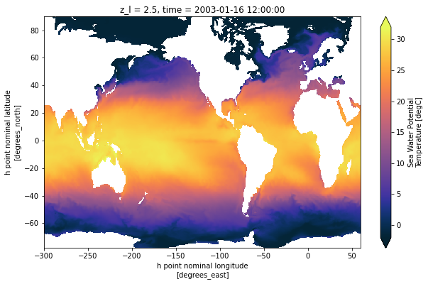
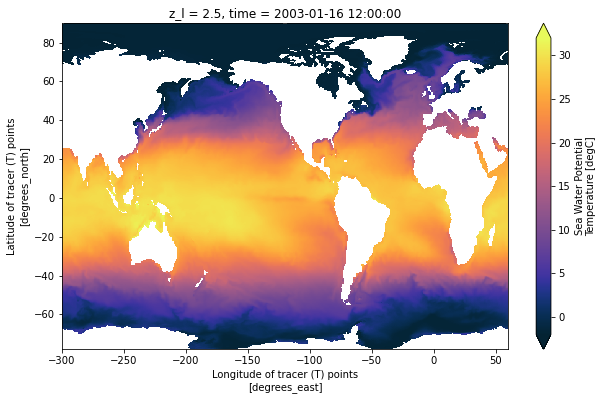
Now notice the difference in the arctic between nominal (bad) coordinates and the true coordinates:

ds['thetao'].isel(time=0, z_l=0).plot(vmin=-2, vmax=32,
                                      cmap=cmocean.cm.thermal,
                                      figsize=[10, 6])

<matplotlib.collections.QuadMesh at 0x7f04a86f0588>

ds['thetao'].isel(time=0, z_l=0).plot(vmin=-2, vmax=32,
                                      x='geolon', y='geolat',
                                      cmap=cmocean.cm.thermal,
                                      figsize=[10, 6])

<matplotlib.collections.QuadMesh at 0x7f04a85bb860>

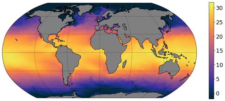
More control on xarray plot

Using the latest xarray >= 0.16.0, you can now adjust plot properties more easily:

plt.figure(figsize=[14, 6])
p = ds['thetao'].isel(time=0, z_l=0).plot(vmin=-2, vmax=32,
                                          x='geolon', y='geolat',
                                          cmap=cmocean.cm.thermal,
                                          subplot_kws={'projection': ccrs.Robinson(),
                                                       'facecolor':'grey'},
                                          transform=ccrs.PlateCarree(),
                                          add_labels=False,
                                          add_colorbar=False)
p.axes.coastlines()
p.axes.gridlines(color='black', alpha=0.5, linestyle='--')

# add separate colorbar
cb = plt.colorbar(p, ticks=[0,5,10,15,20,25,30], shrink=0.95)
cb.ax.tick_params(labelsize=18)

More plotting examples in the plotting section of the cookbook!