Computing Meridional Overturning
Meriodional Overturning Circulation is a key diagnostic for ocean circulation. This notebook demonstrate how to compute various flavors of it using the xoverturning package.
[1]:
import warnings
warnings.filterwarnings('ignore')
[2]:
import numpy as np
import xarray as xr # requires >= 0.15.1
import pandas as pd
from dask.diagnostics import ProgressBar
import matplotlib.pyplot as plt
%matplotlib inline
[3]:
from xoverturning import calcmoc
Load the sample dataset and geolon/geolat from static file (without holes on eliminated processors). Note that this is working for both symetric and non-symetric grids but the dataset and grid file must be consistent.
dataurl = 'http://35.188.34.63:8080/thredds/dodsC/OM4p5/'

ds = xr.open_dataset(f'{dataurl}/ocean_monthly_z.200301-200712.nc4',
                     chunks={'time':1, 'z_l': 1}, engine='pydap')
[4]:
root = '/work/noaa/gfdlscr/jkrastin/wmt-inert-tracer/OM4p5_sample/'
ds = xr.open_dataset(root+'ocean_monthly_z.200301-200712.nc4', chunks={'time':1, 'z_l': 1},
                     drop_variables=['average_DT','average_T1','average_T2'])
[5]:
#dsgrid = xr.open_dataset('./data/ocean_grid_nonsym_OM4_05.nc')
dsgrid = xr.open_dataset('../MOM6-AnalysisCookbook/ocean_grid_nonsym_OM4_05.nc')
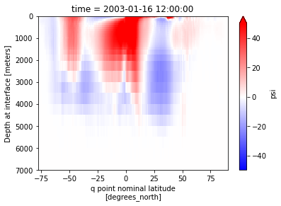
A first overturning computation
This computes the meridional overturning circulation (moc) on the whole ocean:
[6]:
moc = calcmoc(ds, dsgrid=dsgrid)
generating basin codes
The result is given at the vertical interfaces since the streamfunction is the result of the integration of transports over layers and on the q-point because V-velocities are located on (xh, yq) and integrated over the x-axis.
[7]:
print(moc.dims)
('time', 'z_i', 'yq')
[8]:
# Plot streamfunction for any given time
moc.sel(time='2003-01').plot(vmin=-50,vmax=50, yincrease=False, cmap='bwr')
[8]:
<matplotlib.collections.QuadMesh at 0x7f5a5c6d52d0>
[9]:
with ProgressBar():
    moc_mean = moc.mean('time').load()
[########################################] | 100% Completed | 3min 16.3s
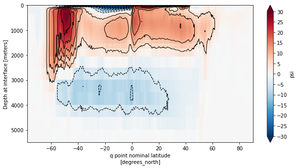
[10]:
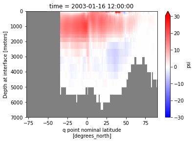
fig, ax = plt.subplots(figsize=(10,5))
moc_mean.plot(ax=ax, yincrease=False,vmin=-30,vmax=30,cmap='RdBu_r',cbar_kwargs={'ticks': np.arange(-30,35,5)})
moc_mean.plot.contour(ax=ax, yincrease=False, levels=np.concatenate([np.arange(-30,0,5),np.arange(5,35,5)]),
                      colors='k', linewidths=1)
ax.set_ylim([5500,0])
plt.show()
MOC and Basins
xoverturning can compute the MOC over a specified basin. Default is basin='global', but pre-defined available options are basin='atl-arc' and basin='indopac'. If the grid file contain a basin DataArray produced by cmip_basins, it will use it in combination with predefined basin codes to create the basin mask. If the array does not exist, xoverturning will generate it on-the-fly using cmip_basin code. It is also possible to use an
arbitrary list of basin codes as argument to basin, which could be particularly handy if you have custom build basin codes.
[11]:
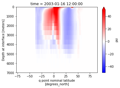
# atlantic
amoc = calcmoc(ds, dsgrid=dsgrid, basin='atl-arc')
generating basin codes
[12]:
amoc.sel(time='2003-01').plot(vmin=-30,vmax=30, yincrease=False, cmap='bwr')
[12]:
<matplotlib.collections.QuadMesh at 0x7f5a3dee9310>
[13]:
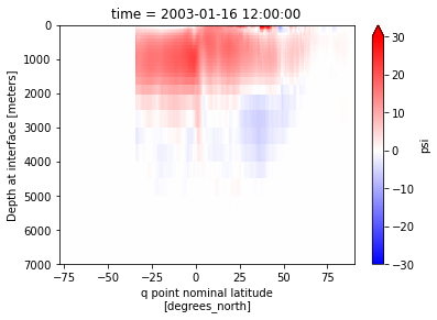
# indopacific
pmoc = calcmoc(ds, dsgrid=dsgrid, basin='indopac')
generating basin codes
[14]:
pmoc.sel(time='2003-01').plot(vmin=-50,vmax=50, yincrease=False, cmap='bwr')
[14]:
<matplotlib.collections.QuadMesh at 0x7f5a4cb84610>
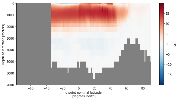
Masking (only in geopotential coordinates)
You can also mask out the ocean floor to make it more plot-friendly with mask_output.
[15]:
amoc = calcmoc(ds, dsgrid=dsgrid, basin='atl-arc', mask_output=True)
generating basin codes
[16]:
amoc.sel(time='2003-01').plot(vmin=-30,vmax=30, yincrease=False, cmap='bwr',
                              subplot_kws={'facecolor': 'grey'})
[16]:
<matplotlib.collections.QuadMesh at 0x7f5a5c2b6590>
[17]:
with ProgressBar():
    amoc_mean = amoc.mean('time').load()
[########################################] | 100% Completed | 2min 19.8s
[18]:
fig, ax = plt.subplots(figsize=(10,5))
amoc_mean.plot(ax=ax, yincrease=False,cmap='RdBu_r',cbar_kwargs={'ticks': np.arange(-30,35,5)})
ax.set_facecolor('grey')
plt.show()
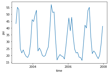
Derived quantities
Since the output of xoverturning is a xarray.DataArray, computing derived quantities is a breeze thanks to xarray built-in functions:
[19]:
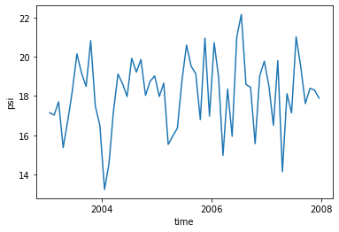
amoc.max(dim=['yq', 'z_i']).plot()
[19]:
[<matplotlib.lines.Line2D at 0x7f5a5422fa50>]
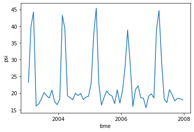
[20]:
amoc.sel(yq=slice(20.0, 80.0), z_i=slice(100.0, 2500.0)).max(dim=['yq', 'z_i']).plot()
[20]:
[<matplotlib.lines.Line2D at 0x7f5a3cc1fb90>]
[21]:
amoc.sel(yq=slice(20.0, 80.0), z_i=slice(500.0, 2500.0)).max(dim=['yq', 'z_i']).plot()
[21]:
[<matplotlib.lines.Line2D at 0x7f5a4c1fc190>]
[22]:
# Find the location of the maximum
yq_max = amoc_mean.argmax(dim=['yq', 'z_i'])['yq']
z_i_max = amoc_mean.argmax(dim=['yq', 'z_i'])['z_i']
print('Maximum:',
      np.round(amoc_mean[z_i_max,yq_max].values,1),'Sv at',
      np.round(amoc_mean.yq[yq_max].values,1),'N and',
      np.round(amoc_mean.z_i[z_i_max].values,1),'m depth')
Maximum: 19.9 Sv at 20.9 N and 15.0 m depth
[23]:
subset = amoc_mean.sel(yq=slice(20.0, 80.0), z_i=slice(100.0, 2500.0))
yq_max = subset.argmax(dim=['yq', 'z_i'])['yq']
z_i_max = subset.argmax(dim=['yq', 'z_i'])['z_i']
[24]:
print('Maximum:',
      np.round(subset[z_i_max,yq_max].values,1),'Sv at',
      np.round(subset.yq[yq_max].values,1),'N and',
      np.round(subset.z_i[z_i_max].values,1),'m depth')
Maximum: 17.0 Sv at 30.0 N and 650.0 m depth
Density coordinates
Because xoverturning is written in a non-specific vertical coordinate system, it can also compute the MOC in other coordinates system, such as the rho2 output by using the vertical='rho2' option.
pproot = '/archive/Raphael.Dussin/FMS2019.01.03_devgfdl_20201120/'
run = 'CM4_piControl_c96_OM4p25_half_kdadd'
ppdir = f'{pproot}/{run}/gfdl.ncrc4-intel18-prod-openmp/pp/ocean_annual_rho2'

ds_rho2 = xr.open_mfdataset([f"{ppdir}/ts/annual/10yr/ocean_annual_rho2.0021-0030.umo.nc",
                             f"{ppdir}/ts/annual/10yr/ocean_annual_rho2.0021-0030.vmo.nc"])

dsgrid_rho2 = xr.open_dataset(f"{ppdir}/ocean_annual_rho2.static.nc")
[25]:
ppdir = '/work/noaa/gfdlscr/jkrastin/wmt-inert-tracer/OTSFN_sample/'
ds_rho2 = xr.open_mfdataset(ppdir+'ocean_annual_rho2.0021-0030.*.nc',
                            drop_variables=['average_DT','average_T1','average_T2'])
[26]:
dsgrid_p25 = xr.open_dataset(ppdir[:-13]+'data/raw/CM4_piControl_C/ocean_monthly/ocean_monthly.static.nc')
[27]:
ds_rho2 = ds_rho2.isel(yq=slice(1,None),xq=slice(1,None))
Global overturning in density coordinates
[28]:
moc_rho2 = calcmoc(ds_rho2, dsgrid=dsgrid_p25, vertical='rho2')
generating basin codes
[29]:
with ProgressBar():
    moc_rho2_mean = moc_rho2.mean('time').load()
[########################################] | 100% Completed | 10.2s
[30]:
fig, ax = plt.subplots(figsize=(10,5))
moc_rho2_mean.sel(rho2_i=slice(1028.5,None)).plot(ax=ax, yincrease=False,vmin=-30,vmax=30,cmap='RdBu_r',
                                                  cbar_kwargs={'ticks': np.arange(-30,35,5)})
moc_rho2_mean.sel(rho2_i=slice(1028.5,None))\
    .plot.contour(ax=ax, yincrease=False, levels=np.concatenate([np.arange(-30,0,5),np.arange(5,35,5)]),
                  colors='k', linewidths=1)
plt.show()
AMOC in density coordinates
[31]:
amoc_rho2 = calcmoc(ds_rho2,dsgrid=dsgrid_p25, vertical='rho2', basin='atl-arc')
generating basin codes
[32]:
with ProgressBar():
    amoc_rho2_mean = amoc_rho2.mean('time').load()
[########################################] | 100% Completed | 10.2s
[33]:
# Find the location of the maximum
yq_max = amoc_rho2_mean.argmax(dim=['rho2_i', 'yq'])['yq']
rho2_i_max = amoc_rho2_mean.argmax(dim=['rho2_i', 'yq'])['rho2_i']
print('Maximum:',
      np.round(amoc_rho2_mean.isel(rho2_i=rho2_i_max,yq=yq_max).values,1),'Sv at',
      np.round(amoc_rho2_mean.yq[yq_max].values,1),'N and',
      np.round(amoc_rho2_mean.rho2_i[rho2_i_max].values,1),'kg/m^3 density')
Maximum: 20.0 Sv at 16.2 N and 1036.7 kg/m^3 density
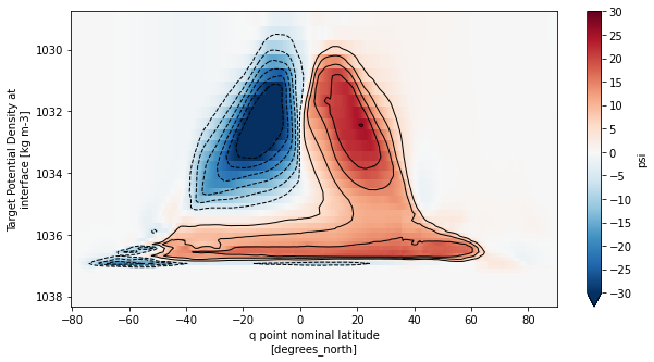
[34]:
fig, ax = plt.subplots(figsize=(10,5))
amoc_rho2_mean.sel(rho2_i=slice(1028.5,None)).plot(ax=ax, yincrease=False,cmap='RdBu_r',
                                                  cbar_kwargs={'ticks': np.arange(-30,35,5)})
amoc_rho2_mean.sel(rho2_i=slice(1028.5,None))\
    .plot.contour(ax=ax, yincrease=False, levels=np.concatenate([np.arange(-20,0,2),np.arange(5,22,2)]),
                  colors='k', linewidths=1)
# Plot location of maximum
ax.plot(amoc_rho2_mean.yq[yq_max],amoc_rho2_mean.rho2_i[rho2_i_max],marker='+',c='m',ms=15,mew=2)
plt.show()
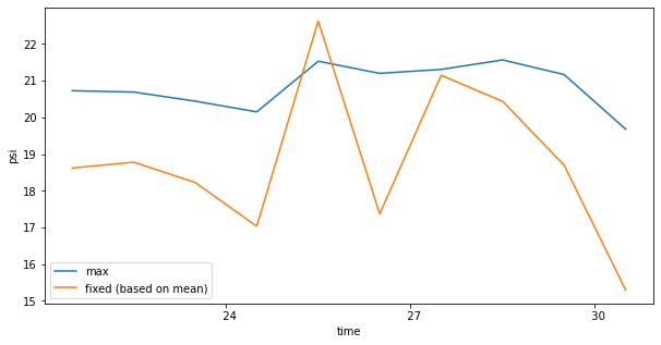
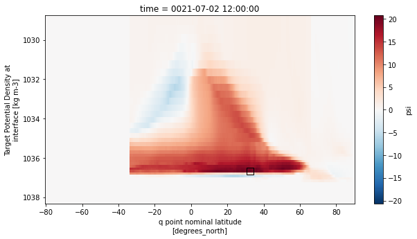
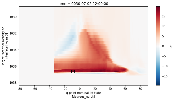
Temporal variability in AMOC
[35]:
fig, ax = plt.subplots(figsize=(10,5))
amoc_rho2.max(dim=['rho2_i', 'yq']).plot(ax=ax,label='max')
moc_rho2.isel(rho2_i=rho2_i_max,yq=yq_max).plot(ax=ax,label='fixed (based on mean)',_labels=None)
ax.legend(loc='lower left')
[35]:
<matplotlib.legend.Legend at 0x7f5a54065ed0>
[36]:
df = pd.DataFrame({'MOC_max': amoc_rho2.max(dim=['rho2_i', 'yq']).values,
                   'rho2_max': amoc_rho2.rho2_i[amoc_rho2.argmax(dim=['rho2_i', 'yq'])['rho2_i'].values],
                   'yq_max': amoc_rho2.yq[amoc_rho2.argmax(dim=['rho2_i', 'yq'])['yq'].values]},
                  columns=['MOC_max', 'rho2_max','yq_max'])
print(df)
     MOC_max   rho2_max     yq_max
0  20.726299  1036.6875  32.691579
1  20.688719  1036.6875  28.166723
2  20.441734  1036.6875  46.311188
3  20.150070  1036.5625  36.195427
4  21.529745  1036.6875  13.255155
5  21.198574  1036.5625  36.998263
6  21.306437  1036.6875  16.636192
7  21.564934  1036.6875  48.840297
8  21.165529  1036.6875  18.779436
9  19.679716  1036.6875  -9.086668
[37]:
fig, ax = plt.subplots(figsize=(10,5))

amoc_rho2[0].sel(rho2_i=slice(1028.5,None)).plot(ax=ax, yincrease=False,cmap='RdBu_r')
ax.plot(df.iloc[0,2],df.iloc[0,1],marker='s',c='k',ms=10,mew=1,mfc='none')
plt.show()
[38]:
fig, ax = plt.subplots(figsize=(10,5))

amoc_rho2[9].sel(rho2_i=slice(1028.5,None)).plot(ax=ax, yincrease=False,cmap='RdBu_r')
ax.plot(df.iloc[9,2],df.iloc[9,1],marker='s',c='k',ms=10,mew=1,mfc='none')
plt.show()
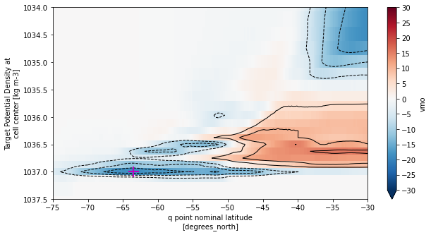
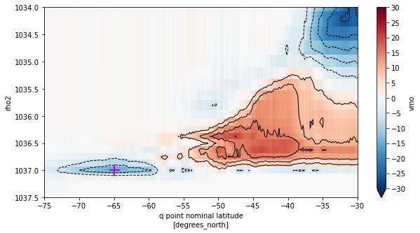
Southern Ocean MOC in density coordinates
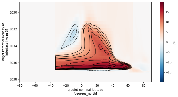
[39]:
rho0 = 1035.0
[40]:
# Calculate streamfunction
vmo_so = ds_rho2.vmo.where(ds_rho2.vmo<1e14).sel(rho2_l=slice(1033,1038),yq=slice(-80,0))
psi_so = (vmo_so.sum('xh').cumsum('rho2_l') - vmo_so.sum('xh').sum('rho2_l'))/rho0/1.0e6 + 0.1
Note conversion from kg s\(^{-1}\) to Sv (10\(^6\) m\(^3\) s\(^{-1}\)):
\[\frac{\psi}{\rho_0 10^6}\]
[41]:
with ProgressBar():
    smoc_rho2_mean = psi_so.mean('time').load()
[########################################] | 100% Completed | 9.4s
[42]:
# Find the location of the minimum (lower limb overturning)
smoc_lower_mean = smoc_rho2_mean.sel(rho2_l=slice(1028.5,None),yq=slice(None,-30))
yq_min_idx = smoc_lower_mean.argmin(dim=['rho2_l', 'yq'])['yq']
rho2_min_idx = smoc_lower_mean.argmin(dim=['rho2_l', 'yq'])['rho2_l']
print('Minimum:',
      np.round(smoc_lower_mean.isel(rho2_l=rho2_min_idx,yq=yq_min_idx).values,1),'Sv at',
      np.round(smoc_lower_mean.yq[yq_min_idx].values,1),'N and',
      np.round(smoc_lower_mean.rho2_l[rho2_min_idx].values,1),'kg/m^3 density')
Minimum: -19.1 Sv at -63.5 N and 1037.0 kg/m^3 density
[43]:
fig, ax = plt.subplots(figsize=(10,5))

smoc_rho2_mean.plot(ax=ax, yincrease=False,vmin=-30,vmax=30,cmap='RdBu_r',
                    cbar_kwargs={'ticks': np.arange(-30,35,5)})
smoc_rho2_mean.plot.contour(ax=ax, yincrease=False, levels=np.concatenate([np.arange(-30,0,5),np.arange(5,35,5)]),
                            colors='k', linewidths=1)
# Plot location of minimum
ax.plot(smoc_lower_mean.yq[yq_min_idx],smoc_lower_mean.rho2_l[rho2_min_idx],marker='+',c='m',ms=15,mew=2)
ax.set_xlim((-75,-30))
ax.set_ylim((1037.5,1034))
plt.show()
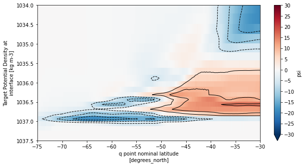
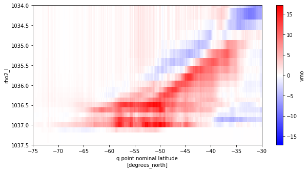
Compare streamfunction to the version obtained from xoverturning
[44]:
fig, ax = plt.subplots(1,1, figsize=(10,5))
moc_rho2_mean.sel(rho2_i=slice(1033,1038),yq=slice(-80,0)).plot(ax=ax, yincrease=False,vmin=-30,vmax=30,cmap='RdBu_r',
                    cbar_kwargs={'ticks': np.arange(-30,35,5)})
moc_rho2_mean.sel(rho2_i=slice(1033,1038),yq=slice(-80,0))\
    .plot.contour(ax=ax, yincrease=False, levels=np.concatenate([np.arange(-30,0,5),np.arange(5,35,5)]),
                  colors='k', linewidths=1)

ax.set_xlim((-75,-30))
ax.set_ylim((1037.5,1034))
plt.show()
Remap meridional transport to density coordinates
Ideally, computation should use vmo from rho2 output, but it is possible to use output in z coordinates and compute the isopycnal overturning offline by first vertically remapping the meridional transport from depth to density levels.
Here, we can use xgcm (in particular the transform method) to compute the isopycnal overturning offline and then compare it to the online rho2 coordinate overturning.
We will focus here on the Southern Ocean MOC. Let’s start by loading the relevant data on the z grid and defining and xgcm grid object.
Load data and build an xgcm grid object
[45]:
ds_z = xr.open_mfdataset(ppdir+'ocean_annual_z.0021-0030.*.nc',
                         drop_variables=['average_DT','average_T1','average_T2'])
[46]:
# Subset dataset to the non-symmetric grid dataset
ds_z = ds_z.isel(yq=slice(1,None),xq=slice(1,None))
[47]:
from xgcm import Grid
[48]:
# Create a pseudo-grid in the vertical
ds_z['dzt'] = xr.DataArray(data=ds_z['z_i'].diff('z_i').values, coords={'z_l': ds_z['z_l']}, dims=('z_l'))
[49]:
# Make sure to fill in NaNs with zeros
ds_z['dxt'] = dsgrid_p25['dxt'].fillna(0.)
ds_z['dyt'] = dsgrid_p25['dyt'].fillna(0.)
ds_z['areacello'] = dsgrid_p25['areacello'].fillna(0.)
ds_z['volcello'] = ds_z['volcello'].fillna(0.)
[50]:
metrics = {
    ('X',): ['dxt'], # X distances
    ('Y',): ['dyt'], # Y distances
    ('Z',): ['dzt'], # Z distances
    ('X', 'Y'): ['areacello'], # Areas
    ('X', 'Y', 'Z'): ['volcello'], # Volumes
}

coords={'X': {'center': 'xh', 'right': 'xq'},
        'Y': {'center': 'yh', 'right': 'yq'},
        'Z': {'center': 'z_l', 'outer': 'z_i'}}
[51]:
xgrid = Grid(ds_z, coords=coords, metrics=metrics, periodic=['X'])
Density field
We also need a density field to which we remap the meridional transport variable vmo. There are several python packages for computations using the Equation Of State (e.g., gsw or xgcm/fastjmd95). To stay consistent with MOM6, one would use the Wright 97 EOS model. The example below will use fastjmd95 to calculate potential density referenced at 2000 dbar.
[52]:
import fastjmd95 as jmd95
[53]:
ds_z['rho2'] = jmd95.rho(ds_z.so, ds_z.thetao, 2000)
[54]:
from xhistogram.xarray import histogram
[55]:
fig, ax = plt.subplots(1,1, figsize=[10,4])
histogram(ds_z.rho2.isel(time=0), bins = [np.linspace(1028, 1038, 101)], density=True).plot(ax=ax,lw=2,c='k')
for val in ds_rho2.rho2_i.values[1:]:
    ax.axvline(x=val,lw=1,alpha=0.5)
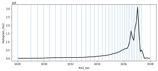
Given the fairly skewed distribution of density towards high values it makes sense to define a density axis with more refined spacing in the high density ranges.
[56]:
# Define density axis
rho2_axis = ds_rho2.rho2_i.values
Remap vmo with xgcm.transform
[57]:
vmo = ds_z.vmo.where(dsgrid_p25['wet_v']==1)
[58]:
# Interpolate density values to vmo grid
rho2 = xgrid.interp(ds_z.rho2, 'Y', boundary='extend').rename('rho2').chunk({'z_l':-1})
[59]:
# Transform into sigma1 coords
vmo_rho2 = xgrid.transform(vmo.chunk({'z_l':-1}), target = rho2_axis, target_data=rho2,
                           method='conservative', mask_edges=True, suffix='_transformed', axis = 'Z')
[60]:
# Check if density coodinated of remapped data is the same as in the original rho2 dataset
pd.DataFrame({'original': ds_rho2.rho2_l.values, 'transform': vmo_rho2.rho2.values},
             columns=['original', 'transform'])
[60]:
| original | transform | |
|---|---|---|
| 0 | 1013.750000 | 1013.750000 |
| 1 | 1028.500000 | 1028.500000 |
| 2 | 1029.242188 | 1029.242188 |
| 3 | 1029.718750 | 1029.718750 |
| 4 | 1030.179688 | 1030.179688 |
| 5 | 1030.625000 | 1030.625000 |
| 6 | 1031.054688 | 1031.054688 |
| 7 | 1031.468750 | 1031.468750 |
| 8 | 1031.867188 | 1031.867188 |
| 9 | 1032.250000 | 1032.250000 |
| 10 | 1032.617188 | 1032.617188 |
| 11 | 1032.968750 | 1032.968750 |
| 12 | 1033.304688 | 1033.304688 |
| 13 | 1033.625000 | 1033.625000 |
| 14 | 1033.929688 | 1033.929688 |
| 15 | 1034.218750 | 1034.218750 |
| 16 | 1034.492188 | 1034.492188 |
| 17 | 1034.750000 | 1034.750000 |
| 18 | 1034.992188 | 1034.992188 |
| 19 | 1035.218750 | 1035.218750 |
| 20 | 1035.429688 | 1035.429688 |
| 21 | 1035.625000 | 1035.625000 |
| 22 | 1035.804688 | 1035.804688 |
| 23 | 1035.968750 | 1035.968750 |
| 24 | 1036.117188 | 1036.117188 |
| 25 | 1036.250000 | 1036.250000 |
| 26 | 1036.375000 | 1036.375000 |
| 27 | 1036.500000 | 1036.500000 |
| 28 | 1036.625000 | 1036.625000 |
| 29 | 1036.750000 | 1036.750000 |
| 30 | 1036.875000 | 1036.875000 |
| 31 | 1037.000000 | 1037.000000 |
| 32 | 1037.125000 | 1037.125000 |
| 33 | 1037.250000 | 1037.250000 |
| 34 | 1037.656250 | 1037.656250 |
[61]:
# Calculate streamfunction
vmo_so_offline = vmo_rho2.where(vmo_rho2<1e14).sel(rho2=slice(1033,1038),yq=slice(-80,0))
psi_so_offline = (vmo_so_offline.sum('xh').cumsum('rho2') - vmo_so_offline.sum('xh').sum('rho2'))/rho0/1.0e6 + 0.1
[62]:
with ProgressBar():
    smoc_rho2_offline_mean = psi_so_offline.mean('time').load()
[########################################] | 100% Completed | 51.2s
[63]:
# Find the location of the minimum (lower limb overturning)
smoc_lower_offline_mean = smoc_rho2_offline_mean.sel(rho2=slice(1028.5,None),yq=slice(None,-50))
yq_min_offline_idx = smoc_lower_offline_mean.argmin(dim=['rho2', 'yq'])['yq']
rho2_min_offline_idx = smoc_lower_offline_mean.argmin(dim=['rho2', 'yq'])['rho2']
print('Minimum:',
      np.round(smoc_lower_offline_mean.isel(rho2=rho2_min_offline_idx,yq=yq_min_offline_idx).values,1),'Sv at',
      np.round(smoc_lower_offline_mean.yq[yq_min_offline_idx].values,1),'N and',
      np.round(smoc_lower_offline_mean.rho2[rho2_min_offline_idx].values,1),'kg/m^3 density')
Minimum: -15.1 Sv at -64.9 N and 1037.0 kg/m^3 density
[64]:
fig, ax = plt.subplots(figsize=(10,5))

smoc_rho2_offline_mean.T.plot(ax=ax, yincrease=False,vmin=-30,vmax=30,cmap='RdBu_r',
                              cbar_kwargs={'ticks': np.arange(-30,35,5)})
smoc_rho2_offline_mean.T\
    .plot.contour(ax=ax, yincrease=False, levels=np.concatenate([np.arange(-30,0,5),np.arange(5,35,5)]),
                  colors='k', linewidths=1)
# Plot location of minimum
ax.plot(smoc_lower_offline_mean.yq[yq_min_offline_idx],smoc_lower_offline_mean.rho2[rho2_min_offline_idx],
        marker='+',c='m',ms=15,mew=2)
ax.set_xlim((-75,-30))
ax.set_ylim((1037.5,1034))
plt.show()
[65]:
# Difference between offline and online
delta = smoc_rho2_offline_mean.T.rename({'rho2':'rho2_l'}) - smoc_rho2_mean
[66]:
fig, ax = plt.subplots(figsize=(10,5))
delta.plot(ax=ax, yincrease=False,cmap='bwr')
ax.set_xlim((-75,-30))
ax.set_ylim((1037.5,1034))
plt.show()
[67]:
smoc_lower_online = psi_so.sel(rho2_l=slice(1028.5,None),yq=slice(None,-50))
smoc_lower_offline = psi_so_offline.sel(rho2=slice(1028.5,None),yq=slice(None,-50))
[68]:
df = pd.DataFrame({
    'Min (online)': smoc_lower_online.min(dim=['rho2_l', 'yq']).values,
    'Min (offline)': smoc_lower_offline.min(dim=['rho2', 'yq']).values,
    'rho2_min_online': smoc_lower_online.rho2_l[smoc_lower_online.argmin(dim=['rho2_l', 'yq'])['rho2_l'].values],
    'rho2_min_offline': smoc_lower_offline.rho2[smoc_lower_offline.argmin(dim=['rho2', 'yq'])['rho2'].values],
    'yq_min_online': smoc_lower_online.yq[smoc_lower_online.argmin(dim=['rho2_l', 'yq'])['yq'].values],
    'yq_min_offline': smoc_lower_offline.yq[smoc_lower_offline.argmin(dim=['rho2', 'yq'])['yq'].values]},
    columns=['Min (online)', 'Min (offline)','rho2_min_online','rho2_min_offline','yq_min_online','yq_min_offline'])
print(df)
   Min (online)  Min (offline)  rho2_min_online  rho2_min_offline  \
0    -28.495102     -19.482939         1037.000            1037.0
1    -23.202520     -15.596636         1037.000            1037.0
2    -21.443588     -16.027849         1037.000            1037.0
3    -21.286764     -15.204092         1036.875            1037.0
4    -20.924694     -16.823597         1036.875            1037.0
5    -15.922176     -12.753931         1037.000            1037.0
6    -18.509733     -15.922901         1037.000            1037.0
7    -22.771084     -16.349289         1036.625            1037.0
8    -20.515707     -14.393363         1036.625            1037.0
9    -20.653469     -15.485858         1037.000            1037.0

   yq_min_online  yq_min_offline
0     -59.834021      -61.307763
1     -62.715357      -63.728938
2     -62.715357      -65.857156
3     -55.138698      -65.857156
4     -54.995544      -65.340774
5     -51.404080      -65.548558
6     -64.492987      -64.814051
7     -60.579293      -64.814051
8     -57.089577      -64.920230
9     -64.920230      -63.282843
[69]:
fig, ax = plt.subplots(figsize=(10,5))
psi_so.sel(rho2_l=slice(1028.5,None))[0].plot(ax=ax, yincrease=False,cmap='RdBu_r')
ax.plot(df.iloc[0,4],df.iloc[0,2],marker='s',c='k',ms=10,mew=1,mfc='none')
plt.show()
[70]:
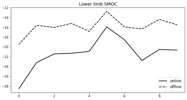
fig, ax = plt.subplots(figsize=(10,5))
df['Min (online)'].plot(ax=ax,label='online',lw=2,c='k')
df['Min (offline)'].plot(ax=ax,label='offline',lw=2,c='k',ls='--')
ax.legend(loc='lower right',fontsize=12)
ax.set_title('Lower limb SMOC',fontsize=14)
plt.show()
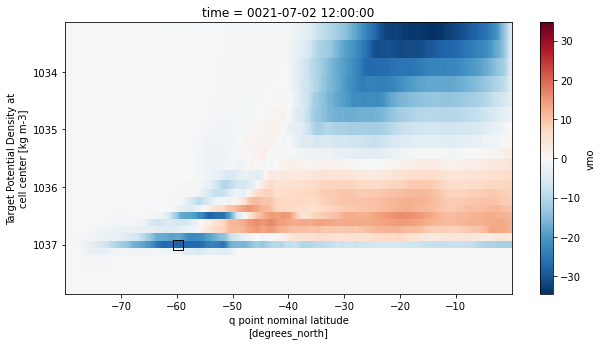
Reproject rho2 overturning to z coordinates
[71]:
thk_p25 = ds_rho2.mean('time').thkcello.values
#thk_p25 = np.ma.masked_greater(thk_p25,1e10)
print(thk_p25.shape,np.ma.is_masked(thk_p25))
(35, 1080, 1440) False
[72]:
# Thickness mapped to rho2
thk = ds_rho2.thkcello.where(ds_rho2.thkcello<1e10).mean('time')

# Cumulative sum of thickness to get the time averaged depth of an isopycnal
zrho = thk.mean('xh').cumsum('rho2_l')
[73]:
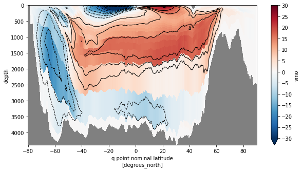
# Calculate streamfunction
vmo = ds_rho2.vmo.where(ds_rho2.vmo<1e14).mean('time')
psi = (vmo.sum('xh').cumsum('rho2_l') - vmo.sum('xh').sum('rho2_l'))/rho0/1.0e6 + 0.1
[74]:
fig, ax = plt.subplots(figsize=(10,5))
psi.plot(ax=ax,x='yq', y='rho2_l',yincrease=False,vmin=-30,vmax=30,cmap='RdBu_r',
                              cbar_kwargs={'ticks': np.arange(-30,35,5)})
psi.plot.contour(ax=ax, yincrease=False, levels=np.concatenate([np.arange(-30,0,5),np.arange(5,35,5)]),
                 colors='k', linewidths=1)
# Plot location of minimum
ax.set_xlim((-75,-30))
ax.set_ylim((1037.5,1034))
ax.set_facecolor('gray')
plt.show()

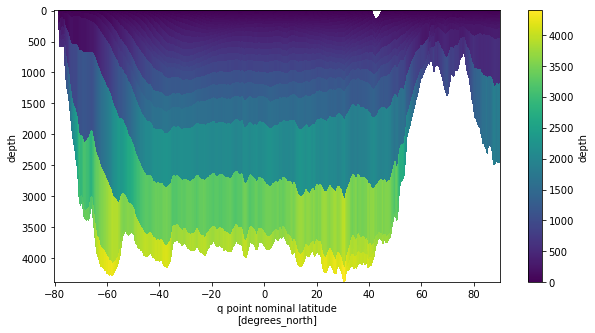
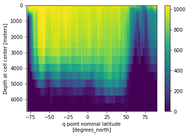
[75]:
psi.coords['depth'] = xgrid.interp(zrho, 'Y', boundary='extend')
[76]:
psi.coords['depth'].plot(x='yq', y='depth',yincrease=False,figsize=(10,5))
[76]:
<matplotlib.collections.QuadMesh at 0x7f5a4c06c910>
[77]:
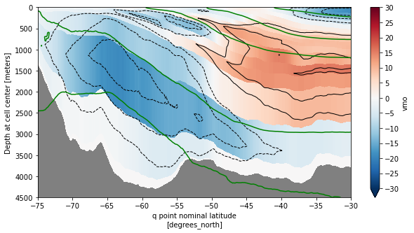
fig, ax = plt.subplots(figsize=(10,5))
psi.plot(ax=ax,x='yq', y='depth',yincrease=False,vmin=-30,vmax=30,cmap='RdBu_r',
                              cbar_kwargs={'ticks': np.arange(-30,35,5)})
psi.plot.contour(ax=ax, x='yq', y='depth', yincrease=False,
                 levels=np.concatenate([np.arange(-30,0,5),np.arange(5,35,5)]),
                 colors='k', linewidths=1)
ax.set_facecolor('gray')
plt.show()
[78]:
with ProgressBar():
    rho_zmean = rho2.mean('time').mean('xh').load()
[########################################] | 100% Completed | 32.0s
[79]:
fig, ax = plt.subplots(figsize=(10,5))
psi.plot(ax=ax,x='yq', y='depth',yincrease=False,vmin=-30,vmax=30,cmap='RdBu_r',
                              cbar_kwargs={'ticks': np.arange(-30,35,5)})
psi.plot.contour(ax=ax, x='yq', y='depth', yincrease=False,
                 levels=np.concatenate([np.arange(-30,0,5),np.arange(5,35,5)]),
                 colors='k', linewidths=1)
rho_zmean.plot.contour(ax=ax,x='yq', y='z_l',yincrease=False,colors='g',lw=2,
                       levels=[1035,1036,1036.5,1037,1037.1])
ax.set_xlim((-75,-30))
ax.set_ylim((4500,0))
ax.set_facecolor('gray')
plt.show()
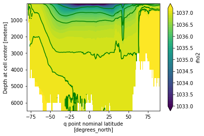
[80]:
rho_zmean.plot.contourf(x='yq', y='z_l',yincrease=False,levels=np.arange(1033,1037.3,0.1))
rho_zmean.plot.contour(x='yq', y='z_l',yincrease=False,colors='g',lw=2,levels=[1035,1036,1036.5,1037,1037.1])
[80]:
<matplotlib.contour.QuadContourSet at 0x7f5a3c83de50>
[81]:
# zonal mean based on MOM6-AnalysisCookbook/docs/notebooks/spatial_operations.ipynb
[82]:
# proper zonal mean
def zonal_mean(da, metrics):
    num = (da * metrics['dxCv'] * metrics['wet_v']).sum(dim=['xh'])
    denom = (metrics['dxCv'] * metrics['wet_v']).sum(dim=['xh'])
    return num/denom
[83]:
with ProgressBar():
    rho2_zm = zonal_mean(rho2.mean('time'),dsgrid_p25).load()
[########################################] | 100% Completed | 32.2s
[84]:
### What went wrong here?
rho2_zm.plot(x='yq', y='z_l',yincrease=False)
[84]:
<matplotlib.collections.QuadMesh at 0x7f5a4c3a7fd0>
[85]:
rho2_zm.where(rho2_zm>0).plot(x='yq', y='z_l',yincrease=False)
[85]:
<matplotlib.collections.QuadMesh at 0x7f5a3df24350>
Misc options
xoverturning also have more specialized options such as remove_hml that is used to remove the signal ov vhml and a rotate option attempting to rotate to true north. This latest option is still in progress and will be updated.